RMS and Summation in Faust
In this tutorial, we present different programming techniques to compute the sum of n consecutive samples in Faust. Such sums are typically used when computing the RMS value of a signal. It is therefore in the RMS context that we will present them. We will not use any predefined function, only Faust primitives, so that you can see all the details.
The text is intended for beginners with some basic knowledge of Faust. If this is not the case, have a look at the various documentations on this website.
RMS value
The computation of the RMS (Root Mean Square) value of a signal is defined by the following Faust expression:
^(2) : summation : /(n) : sqrt
where n is the number of consecutive samples considered.
This expression involves several steps:
- First, we take the square of the signal:
^(2). This is the S of RMS. - Then we sum the n consecutive samples:
summationand divide this sum by n to get the mean value:/(n). This is the M of RMS. - Finally, we take the square root
sqrt. This is the R of RMS.
In other words, RMS is written S:M:R in Faust (leaving the summation function undefined for the moment):
RMS(n) = S:M:R with {
    S = ^(2);
    M = summation : /(n);
    R = sqrt;
};
In the following paragraphs, we will introduce 4 different techniques to write this summation function. We will assume that the audio samples are between -1 and 1.
Sliding Sum
Let's start with the sliding sum approach, probably the simplest way to efficiently add n consecutive samples. First, let's recall that we can add up all the samples of a signal s, from time 0 to the present time, with the following expression: s : +~_.
The trick for adding only the last n samples is to subtract from this sum the same sum but as it was n samples earlier. For example, in order to keep only the sum of the last 10 samples, we just have to subtract from the sum of all samples (s:+~_) the value of this same sum 10 samples ago (s:+~_ : @(10)):
(s:+~_), (s:+~_ : @(10)) : -
This expression can be further simplified by factoring s:+~_. We then get:
s : +~_ <: _, @(10) : -
From a mathematical point of view, this is perfectly correct but poses problems when computed using floating-point numbers. Unlike mathematical numbers, floating-point numbers have a limited precision (23 bits in single precision). When calculating the RMS value, we only add positive numbers. Therefore the sum will increase forever. But at some point, when the sum exceeds , the least significant bit will be higher than any number between and . Therefore adding such a small number will be exactly like adding 0, and the sum will never evolve anymore.
Fortunately, the problem can be solved easily. We just have to swap the integration and the difference parts:
s <: _, @(10) : - : +~_
This new formulation is identical to the previous one from a mathematical point of view. But now, the sum will always stay between and , and the accuracy problems are only on the least significant bits. If the roundoff error due to quantization is modeled as a uniformly distributed random number between -q/2 and q/2, then its variance (mean square) is q^2/12, and this value increases linearly over time in a running sum (see "Wiener process"). Thus, we expect the roundoff error in a running-sum rms calculator to grow proportional to the square root of time.
We can now complete the definition of RMS:
RMS(n) = S:M:R with {
    S = ^(2);
    M = summation : /(n);
    R = sqrt;

    summation = _ <: _, @(n) : - : +~_;
};
Fixed-Point Sliding Sum
While the previous solution works very well with typical signals over practical time spans, the roundoff error continues to grow slowly. To avoid a gradual loss of precision, we can use a fixed-point encoding of the samples, so that the subtraction after delay is always exact. Let's say that we want a sliding sum of 10 values between 0 and 1. We know that this sum will never exceed . We could therefore use up to 27 bits (31-4) to code the fractional part of values.
The conversions are straightforward. To convert floating-point values to fix-point we can use the following expression: *(2^27):int. To convert back from fix-point to floating-point we can use the inverse expression: float:/(2^27).
We can now complete the definition of RMS. As we can see in the summation definition below, we first convert the samples to fix-point, do the summation on integers, then convert the result back to floating-point:
RMS(n) = S:M:R with {
    S = ^(2);
    M = summation : /(n);
    R = sqrt;

    summation = float2fix(16) : _ <: _, @(n) : - : +~_ : fix2float(16);
    float2fix(p) = *(2^p) : int;
    fix2float(p) = float : /(2^p);
};
Obviously this is correct only if we leave enough bits for the integral part. Here we have 15 bits (31-16), enough for n up to 32000 samples.
Block Sum
Sliding sums have a nice and smooth behavior because an updated sum is produced every sample. But they require a large delay line (larger than n), and can have precision problems. In this third approach, we will use a summation by blocks. The summation will be exact, will not require a large delay line, but will be only updated once per block of n samples.
The code is a little bit more involved. It will require a phase signal: , and a capture (sample and hold) operation.
Let's start with a simplified version derived from: s:+~_. Remind that _ is the identity function and is equivalent to *(1). We can therefore rewrite the previous expression s:+~*(1). Now, imagine that instead of 1 we have a boolean b as in: s:~*(b). When b is 1 the input sample is added to the previous sum, but when b is 0 the input sample is added to 0, and the sum is reset to be the input sample.
In our case, we want to reset the sum after every block of n samples, that is, every time phase returns to 0. This can be written: s:+~*(phase!=0).
Note that we can't use the output of this expression directly. It only represents the sum we are looking for when phase==(n-1). That is why we need an additional capture stage to sample the sum and hold it while the next block is processed. Let's say that b indicates when to capture the input value, then: select2(b)~_ will do the job. When b is 0, it reproduces the feedback signal, and when b is 1, it captures the input signal.
Here is the full implementation:
RMS(n) = S:M:R with {
    S = ^(2);
    M = summation : /(n);
    R = sqrt;

    summation = + ~ *(phase != 0) : capture(phase==(n-1));
    phase = 1 : (+,n:%)~_;
    capture(b) = select2(b)~_;
};
Overlapping Block Sum
As we mentioned, the block sum has the disadvantage of producing a new value only once per block. If the blocks are large, this can be a problem. In this fourth approach, we will see how to overlap the produced values. For example, we would like to compute the sum of the last 1000 samples, but with a new result every 250 samples (i.e., an overlap of 75%).
The principle will be to sum small blocks of 250 samples, keep the last four sums, and add them together to produce, every 250 samples, a new sum of the last 1000 samples. Let's call w the size of a small block, and c the number of small blocks in a large block of n samples (i.e., ).
Instead of computing sums of n samples as with: + ~ *(phase != 0), we compute sums of w samples: + ~ *(phase%w != 0). Instead of having one capture every n samples: capture(phase == (n-1)), we need c captures in parallel at 1*w-1, 2*w-1, etc.: par(i,c, capture( phase == (w*(i+1) - 1) ))
Here is the full code:
RMS(n) = S:M:R with {
    S = ^(2);
    M = summation : /(n);
    R = sqrt;

    c = 4; // number of overlaps
    summation = + ~ *(phase%w != 0)
                 <: par(i, c, capture( phase == (w*(i+1) - 1) ))
                 :> _
        with { w = n/c; };

    phase = 1 : (+,n:%)~_;
    capture(b) = select2(b)~_;
};
Comparing all the solutions
Using the Faust IDE, we can easily compare all these solutions. To encapsulate all the definitions and select the RMS implementation, we will use an environment. If you are not familiar with the concept of environment, it is a way to group definitions.

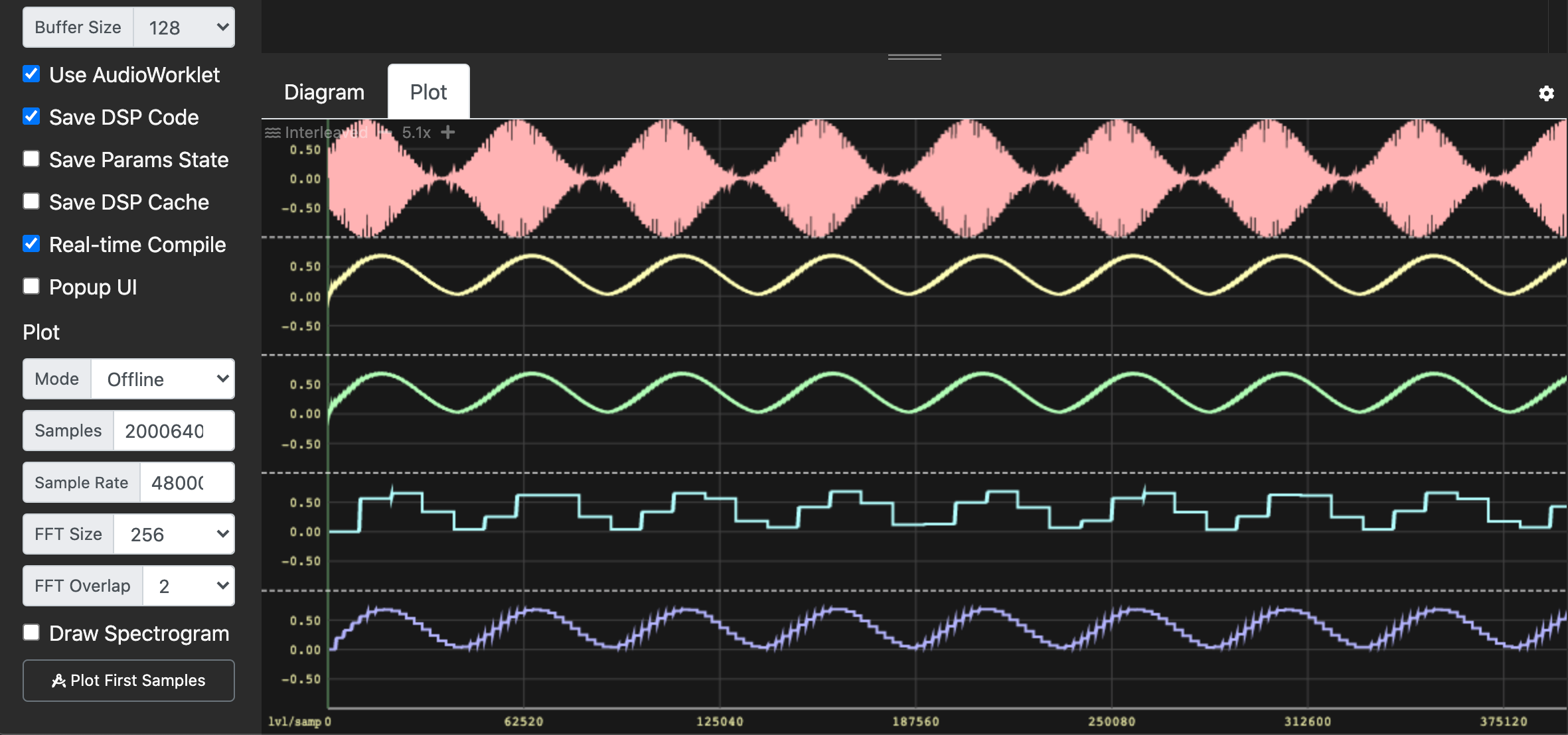
The screenshot of the Faust IDE below shows the RMS values of testsource according to the four methods: Sliding Sum, Fixed-Point Sliding Sum, Block Sum, and Overlapping Block Sum.