
Faust Syntax
Faust Program
A Faust program is essentially a list of statements. These statements can be metadata declarations (either global metadata or function metadata), imports, definitions, and documentation tags, with optional C++-style (//... and /*...*/) comments.
Variants
Some statements (imports, definitions) can be preceded by a variantlist, composed of variants which can be singleprecision, doubleprecision, quadprecision or fixedpointprecision. This allows some imports and definitions to be effective only for a (or several) specific float precision option in the compiler (that is either -single, -double, -quad or -fx respectively). A typical use-case is the definition of floating point constants in the maths.lib library with the following lines:
singleprecision MAX = 3.402823466e+38;
doubleprecision MAX = 1.7976931348623158e+308;
A Simple Program
Here is a short Faust program that implements a simple noise generator (called from the noises.lib Faust library). It exhibits various kinds of statements: two global metadata declarations, an imports, a comment, and a definition. We will study later how documentation statements work:

The keyword process is the equivalent of main in C/C++. Any Faust program, to be valid, must at least define process.
Statements
The statements of a Faust program are of four kinds:
- metadata declarations,
- file imports,
- definitions,
- documentation.
All statements but documentation end with a semicolon ;.
Metadata
Metadata lets us add elements that are not part of the language to Faust code. These can range from the name of a Faust program or its author to potential compilation options or user interface element customizations.
There are three different types of metadata in Faust:
- Global Metadata: metadata global to a Faust code
- Function Metadata: metadata specific to a function
- UI Metadata: metadata specific to a UI element
Note that some Global Metadata have standard names and can be used for specific tasks. Their role is described in the Standard Metadata section.
Global Metadata
All global metadata declarations in Faust start with declare, followed by a key and a string. For example:
declare name "Noise";
allows us to specify the name of a Faust program as a whole.
Unlike regular comments, metadata declarations will appear in the C++ code generated by the Faust compiler. A good practice is to start a Faust program with some standard declarations:
declare name "MyProgram";
declare author "MySelf";
declare copyright "MyCompany";
declare version "1.00";
declare license "BSD";
Function Metadata
Metadata can be associated with a specific function. In that case, declare is followed by the name of the function, a key, and a string. For example:
declare add author "John Doe"
add = +;
This is very useful when a library has several contributors and functions potentially have different license terms, etc.
Standard Metadata
There exists a series of standard global metadata in Faust whose role is described in the following table:
| Metadata | Role |
|---|---|
declare options "[key0:value][key1:value]" |
This metadata can be used to specify various options associated with a Faust code, such as whether it is polyphonic or if it should have OSC, MIDI support, etc. Specific keys usable with this metadata are described throughout this documentation. |
declare interface "xxx" |
Specifies an interface replacing the standard Faust UI. |
Imports
File imports allow us to import definitions from other source files.
For example import("maths.lib"); imports the definitions of the maths.lib library.
The most common file to be imported is the stdfaust.lib library which gives access to all the standard Faust libraries from a single point:

Documentation Tags
Documentation statements are optional and typically used to control the generation of the mathematical documentation of a Faust program. This documentation system is detailed in the Mathematical Documentation chapter. In this section we essentially describe the documentation statements syntax.
A documentation statement starts with an opening <mdoc> tag and ends with a closing </mdoc> tag. Free text content, typically in Latex format, can be placed in between these two tags.

Moreover, optional sub-tags can be inserted in the text content itself to require the generation, at the insertion point, of mathematical equations, graphical block-diagrams, Faust source code listing and explanation notice.

The generation of the mathematical equations of a Faust expression can be requested by placing this expression between an opening <equation> and a closing </equation> tag. The expression is evaluated within the lexical context of the Faust program.

Similarly, the generation of the graphical block-diagram of a Faust expression can be requested by placing this expression between an opening <diagram> and a closing </diagram> tag. The expression is evaluated within the lexical context of the Faust program.

The <metadata> tags allow us to reference Faust global metadata, calling the corresponding keyword.

The <notice/> empty-element tag is used to generate the conventions used in the mathematical equations.

The <listing/> empty-element tag is used to generate the listing of the Faust program. Its three attributes mdoctags, dependencies, and distributed enable or disable respectively <mdoc> tags, other file dependencies, and the distribution of interleaved Faust code between <mdoc> sections.
Definitions
A definition associates an identifier with an expression. Definitions are essentially a convenient shortcut that avoids typing long expressions. During compilation, more precisely during the evaluation stage, identifiers are replaced by their definitions. It is therefore always equivalent to use an identifier or directly its definition. Please note that multiple definitions of the same identifier are not allowed, unless it is a pattern-matching-based definition.
Simple Definitions
The syntax of a simple definition is:
identifier = expression;
For example here is the definition of random, a simple pseudo-random number generator:
random = +(12345) ~ *(1103515245);
Function Definitions
Definitions with formal parameters correspond to functions definitions.
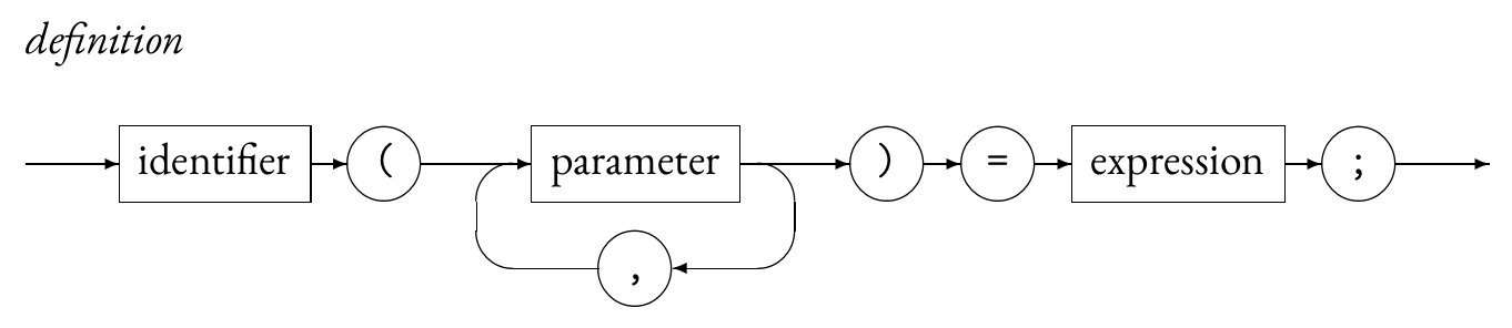
For example the definition of linear2db, a function that converts linear values to decibels, is:
linear2db(x) = 20*log10(x);
Please note that this notation is only a convenient alternative to the direct use of lambda-abstractions (also called anonymous functions). The following is an equivalent definition of linear2db using a lambda-abstraction:
linear2db = \(x).(20*log10(x));
Definitions With Pattern Matching
Moreover, formal parameters can also be full expressions representing patterns:
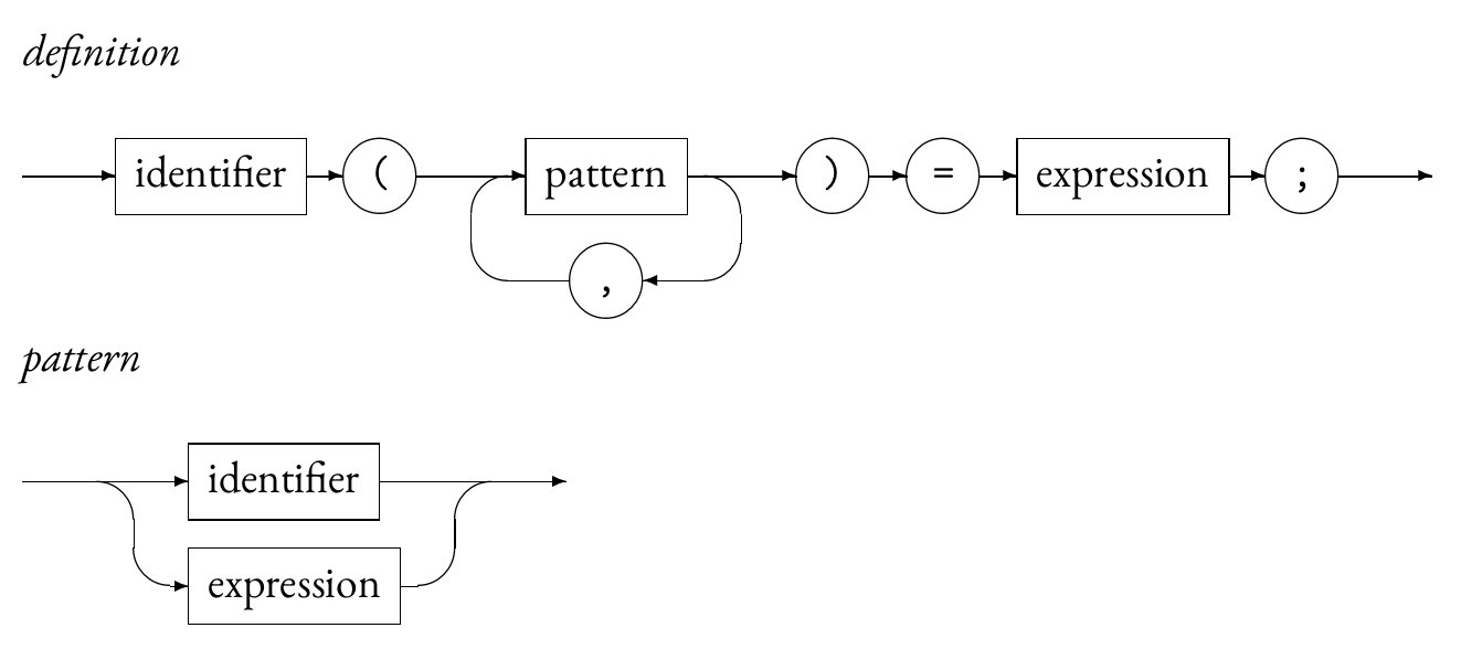
This powerful mechanism allows to algorithmically create and manipulate block diagrams expressions. Let's say that you want to describe a function to duplicate an expression several times in parallel:
duplicate(1,x) = x;
duplicate(n,x) = x, duplicate(n-1,x);
Note that this last definition is a convenient alternative to the more verbose:
duplicate = case {
  (1,x) => x;
  (n,x) => x, duplicate(n-1,x);
};
A use case for duplicate could be to put 5 white noise generators in parallel:

Here is another example to count the number of elements of a list. Please note that we simulate lists using parallel composition: (1,2,3,5,7,11). The main limitation of this approach is that there is no empty list. Moreover lists of only one element are represented by this element:
count((x,xs)) = 1+count(xs);
count(x) = 1;
If we now write count(duplicate(10,666)), the expression will be evaluated as 10.
Note that the order of pattern matching rules matters. The more specific rules must precede the more general rules. When this order is not respected, as in:
count(x) = 1;
count((x,xs)) = 1+count(xs);
the first rule will always match and the second rule will never be called.
Please note that number arguments in pattern matching rules are typically constant numerical expressions, so can be the result of more complex expressions involving computations done at compile-time.
Expressions
Despite its textual syntax, Faust is conceptually a block-diagram language. Faust expressions represent DSP block-diagrams and are assembled from primitive ones using various composition operations. More traditional numerical expressions in infix notation are also possible. Additionally Faust provides time based expressions, like delays, expressions related to lexical environments, expressions to interface with foreign function and lambda expressions.

Constant Numerical Expressions
Some language primitives (like rdtable, rwtable, hslider etc.) take constant numbers as some of their parameters. This is the case also for expressions using pattern matching techniques. Those numbers can be directly given in the code, but can also be computed by more complex expressions which have to produce numbers known at compile time. We will refer to them as constant numerical expressions in the documentation.
Diagram Expressions
Diagram expressions are assembled from primitive ones using either binary composition operations or high level iterative constructions.

Diagram Composition Operations
Five binary composition operations are available to combine block-diagrams:
- recursion (
~), - parallel (
,), - sequential (
:), - split (
<:), - merge (
:>).
One can think of each of these composition operations as a particular way to connect two block diagrams.

To describe precisely how these connections are done, we have to introduce some notation. The number of inputs and outputs of a block-diagram are expressed as and . The inputs and outputs themselves are respectively expressed as: , , , and , , , etc.
For each composition operation between two block-diagrams and we will describe the connections that are created and the constraints on their relative numbers of inputs and outputs.
The priority and associativity of these five operations are:
| Syntax | Priority | Association | Description |
|---|---|---|---|
expression ~ expression |
4 | left | Recursive Composition |
expression , expression |
3 | right | Parallel Composition |
expression : expression |
2 | right | Sequential Composition |
expression <: expression |
1 | right | Split Composition |
expression :> expression |
1 | right | Merge Composition |
Please note that a higher priority value means a higher priority in the evaluation order. There is a companion table that gives the associativity of each numerical operator in infix expressions.
Parallel Composition
The parallel composition (e.g., (A,B)) is probably the simplest one. It places the two block-diagrams one on top of the other, without connections. The inputs of the resulting block-diagram are the inputs of A and B. The outputs of the resulting block-diagram are the outputs of A and B.
Parallel composition is an associative operation: (A,(B,C)) and ((A,B),C) are equivalent. When no parentheses are used (e.g., A,B,C,D), Faust uses right associativity and therefore builds internally the expression (A,(B,(C,D))). This organization is important to know when using pattern matching techniques on parallel compositions.
Example: Oscillators in Parallel
Parallel composition can be used to put 3 oscillators of different kinds and frequencies in parallel, which will result in a Faust program with 3 outputs:

Example: Stereo Effect
Parallel composition can be used to easily turn a mono effect into a stereo one which will result in a Faust program with 2 inputs and 2 outputs:

Note that there's a better to write this last example using the par iteration:

Sequential Composition
The sequential composition (e.g., A:B) expects:
It connects each output of to the corresponding input of :
Sequential composition is an associative operation: (A:(B:C)) and ((A:B):C) are equivalent. When no parentheses are used, like in A:B:C:D, Faust uses right associativity and therefore builds internally the expression (A:(B:(C:D))).
Example: Sine Oscillator
Since everything is considered as a signal generator in Faust, sequential composition can be simply used to pass an argument to a function:

Example: Effect Chain
Sequential composition can be used to create an audio effect chain. Here we're plugging a guitar distortion to an autowah:

Split Composition
The split composition (e.g., A<:B) operator is used to distribute the outputs of to the inputs of .
For the operation to be valid, the number of inputs of must be a multiple of the number of outputs of :
Each input of is connected to the output of :
Example: Duplicating the Output of an Oscillator
Split composition can be used to duplicate signals. For example, the output of the following sawtooth oscillator is duplicated three times in parallel.

Note that this can be written in a more effective way by replacing _,_,_ with par(i,3,_) using the par iteration.
Example: Connecting a Mono Effect to a Stereo One
More generally, the split composition can be used to connect a block with a certain number of outputs to a block with a greater number of inputs:

Note that an arbitrary number of signals can be split, for example:

Once again, the only rule here is that in the expression A<:B the number of inputs of B has to be a multiple of the number of outputs of A.
Merge Composition
The merge composition (e.g., A:>B) is the dual of the split composition. The number of outputs of must be a multiple of the number of inputs of :
Each output of is connected to the input of :
The incoming signals of an input of are summed together.
Example: Summing Signals Together - Additive Synthesis
Merge composition can be used to sum an arbitrary number of signals together. Here's an example of a simple additive synthesizer (note that the result of the sum of the signals is divided by three to prevent clicking):

While the resulting block diagram will look slightly different, this is mathematically equivalent to:

Example: Connecting a Stereo Effect to a Mono One
More generally, the merge composition can be used to connect a block with a certain number of outputs to a block with a smaller number of inputs:

Note that an arbitrary number of signals can be split, for example:

Once again, the only rule with this is that in the expression A:>B the number of outputs of A has to be a multiple of the number of inputs of B.
Recursive Composition
The recursive composition (e.g., A~B) is used to create cycles in the block-diagram in order to express recursive computations. It is the most complex operation in terms of connections.
To be applicable, it requires that:
Each input of is connected to the corresponding output of via an implicit 1-sample delay:
and each output of is connected to the corresponding input of :
The inputs of the resulting block diagram are the remaining unconnected inputs of . The outputs are all the outputs of .
Example: Timer
Recursive composition can be used to implement a "timer" that will count each sample starting at time :

The difference equation corresponding to this program is:
an its output signal will look like: .
Example: One Pole Filter
Recursive composition can be used to implement a one pole filter with one line of code and just a few characters:

The difference equation corresponding to this program is:
Note that the one sample delay of the filter is implicit here so it doesn't have to be declared.
Inputs and Outputs of an Expression
The number of inputs and outputs of a Faust expression can be known at compile time simply by using inputs(expression) and outputs(expression).
For example, the number of outputs of a sine wave oscillator can be known simply by writing the following program:

Note that Faust automatically simplified the expression by generating a program that just outputs 1.
This type of construction is useful to define high order functions and build algorithmically complex block-diagrams. Here is an example to automatically reverse the order of the outputs of an expression.
Xo(expr) = expr <: par(i,n,ba.selector(n-i-1,n))
with {
  n = outputs(expr);
};
And the inputs of an expression:
Xi(expr) = si.bus(n) <: par(i,n,ba.selector(n-i-1,n)) : expr
with {
  n = inputs(expr);
};
For example Xi(-) will reverse the order of the two inputs of the subtraction:

Iterations
Iterations are analogous to for(...) loops in other languages and provide a convenient way to automate some complex block-diagram constructions.

The use and role of par, seq, sum, and prod are detailed in the following sections.
par Iteration
The par iteration can be used to duplicate an expression in parallel. Just like other types of iterations in Faust:
- its first argument is a variable name containing the number of the current iteration (a bit like the variable that is usually named
iin a for loop) starting at 0, - its second argument is the number of iterations, as an integer constant numerical expression, automatically promoted to int
- its third argument is the expression to be duplicated.
Example: Simple Additive Synthesizer

i is used here at each iteration to compute the value of the frequency of the current oscillator. Also, note that this example could be rewritten using sum iteration (see example in the corresponding section).
seq Iteration
The seq iteration can be used to duplicate an expression in series. Just like other types of iterations in Faust:
- its first argument is a variable name containing the number of the current iteration (a bit like the variable that is usually named
iin a for loop) starting at 0, - its second argument is the number of iterations, as an integer constant numerical expression, automatically promoted to int
- its third argument is the expression to be duplicated.
Example: Peak Equalizer
The fi.peak_eq function of the Faust libraries implements a second order "peak equalizer" section (gain boost or cut near some frequency). When placed in series, it can be used to implement a full peak equalizer:

Note that i is used here at each iteration to compute various elements and to format some labels. Having user interface elements with different names is a way to force their differentiation in the generated interface.
sum Iteration
The sum iteration can be used to duplicate an expression as a sum. Just like other types of iterations in Faust:
- its first argument is a variable name containing the number of the current iteration (a bit like the variable that is usually named
iin a for loop) starting at 0, - its second argument is the number of iterations, as an integer constant numerical expression, automatically promoted to int
- its third argument is the expression to be duplicated.
Example: Simple Additive Synthesizer
The following example is just a slightly different version from the one presented in the par iteration section. While their block diagrams look slightly different, the generated code is exactly the same.

i is used here at each iteration to compute the value of the frequency of the current oscillator.
prod Iteration
The prod iteration can be used to duplicate an expression as a product. Just like other types of iterations in Faust:
- its first argument is a variable name containing the number of the current iteration (a bit like the variable that is usually named
iin a for loop) starting at 0, - its second argument is the number of iterations, as an integer constant numerical expression, automatically promoted to int
- its third argument is the expression to be duplicated.
Example: Amplitude Modulation Synthesizer
The following example implements an amplitude modulation synthesizer using an arbitrary number of oscillators thanks to the prod iteration:

i is used here at each iteration to compute the value of the frequency of the current oscillator. Note that the shift parameter can be used to tune the frequency drift between each oscillator.
Infix Notation and Other Syntax Extensions
Infix notation is commonly used in mathematics. It consists in placing the operand between the arguments as in
Besides its algebra-based core syntax, Faust provides some syntax extensions, in particular the familiar infix notation. For example if you want to multiply two numbers, say 2 and 3, you can write directly 2*3 instead of the equivalent core-syntax expression 2,3 : *.
The infix notation is not limited to numbers or numerical expressions. Arbitrary expressions A and B can be used, provided that A,B has exactly two outputs. For example _/2 is equivalent to _,2:/ which divides the incoming signal by 2.
Here are a few examples of equivalences:
| Infix Syntax | Core Syntax | |
|---|---|---|
2-3 |
2,3 : - |
|
2*3 |
2,3 : * |
|
_@7 |
_,7 : @ |
|
_/2 |
_,2 : / |
|
A<B |
A,B : < |
In case of doubts on the meaning of an infix expression, for example _*_, it is useful to translate it to its core syntax equivalent, here _,_:*, which is equivalent to *.
Infix Operators
Built-in primitives that can be used in infix notation are called infix operators and are listed below. Please note that a more detailed description of these operators is available section on primitives.

Comparison Operators
Comparison operators compare two signals and produce a signal that is 1 when the comparison is true and 0 when the comparison is false. The priority and associativity of the comparison operators is given here:
| Syntax | Pri. | Assoc. | Description |
|---|---|---|---|
expression < expression |
5 | left | less than |
expression <= expression |
5 | left | less or equal |
expression == expression |
5 | left | equal |
expression != expression |
5 | left | different |
expression >= expression |
5 | left | greater or equal |
expression > expression |
5 | left | greater than |
Math Operators
Math operators combine two signals and produce a resulting signal by applying a numerical operation on each sample. The priority and associativity of the comparison operators is given here:
| Syntax | Pri. | Assoc. | Description |
|---|---|---|---|
expression + expression |
6 | left | addition |
expression - expression |
6 | left | subtraction |
expression * expression |
7 | left | multiplication |
expression / expression |
7 | left | division |
expression % expression |
7 | left | modulo |
expression ^ expression |
8 | left | power |
Bitwise Operators
Bitwise operators combine two signals and produce a resulting signal by applying a bitwise operation on each sample. The priority and associativity of the bitwise operators is given here:
| Syntax | Pri. | Assoc. | Description |
|---|---|---|---|
expression | expression |
6 | left | bitwise or |
expression & expression |
7 | left | bitwise and |
expression xor expression |
7 | left | bitwise xor |
expression << expression |
7 | left | bitwise left shift |
expression >> expression |
7 | left | bitwise right shift |
Delay operators
Delay operators combine two signals and produce a resulting signal by applying a bitwise operation on each sample. The delay operator @ allows to delay left handside expression by the amount defined by the right handside expression. The unary operator ’ delays the left handside expression by one sample.
| Syntax | Pri. | Assoc. | Description |
|---|---|---|---|
expression @ expression |
9 | left | variable delay |
expression' |
10 | left | one-sample delay |
Prefix Notation
Beside infix notation, it is also possible to use prefix notation. The prefix notation is the usual mathematical notation for functions , but extended to infix operators.
It consists in first having the operator, for example /, followed by its arguments between parentheses: /(2,3):
| Prefix Syntax | Core Syntax | |
|---|---|---|
*(2,3) |
2,3 : * |
|
@(_,7) |
_,7 : @ |
|
/(_,2) |
_,2 : / |
|
<(A,B) |
A,B : < |
Partial Application
The partial application notation is a variant of the prefix notation in which not all arguments are given. For instance /(2) (divide by 2), ^(3) (rise to the cube), and @(512) (delay by 512 samples) are examples of partial applications where only one argument is given. The result of a partial application is a function that "waits" for the remaining arguments.
When doing partial application with an infix operator, it is important to note that the supplied argument is not the first argument, but always the second one:
| Prefix Partial Application Syntax | Core Syntax | |
|---|---|---|
+(C) |
_,C : + |
|
-(C) |
_,C : - |
|
<(C) |
_,C : < |
|
/(C) |
_,C : / |
For commutative operations that doesn't matter. But for non-commutative ones, it is more "natural" to fix the second argument. We use divide by 2 (/(2)) or rise to the cube (^(3)) more often than the other way around.
Please note that this rule only applies to infix operators, not to other primitives or functions. If you partially apply a regular function to a single argument, it will correspond to the first parameter.
Example: Gain Controller
The following example demonstrates the use of partial application in the context of a gain controller:

' Time Expression
' is used to express a one sample delay. For example:

will delay the incoming signal by one sample.
' time expressions can be chained, so the output signal of this program:

will look like: .
The ' time expression is useful when designing filters, etc. and is equivalent to @(1) (see the @ Time Expression).
@ Time Expression
@ is used to express a delay with an arbitrary number of samples. For example:

will delay the incoming signal by 10 samples.
A delay expressed with @ doesn't have to be fixed but it must be bounded and cannot be negative. Therefore, the values of a slider are perfectly acceptable:

@ only allows for the implementation of integer delay. Thus, various fractional delay algorithms are implemented in the Faust delays.lib library.
Environment Expressions
Faust is a lexically scoped language. The meaning of a Faust expression is determined by its context of definition (its lexical environment) and not by its context of use.
To keep their original meaning, Faust expressions are bounded to their lexical environment in structures called closures. The following constructions allow to explicitly create and access such environments. Moreover they provide powerful means to reuse existing code and promote modular design.

with Expression
The with construction allows to specify a local environment: a private list of definition that will be used to evaluate the left hand expression.
In the following example:

the definitions of f(x) and g(x) are local to f : + ~ g.
Please note that with is left associative and has the lowest priority:
f : + ~ g with {...}is equivalent to(f : + ~ g) with {...}.f : + ~ g with {...} with {...}is equivalent to((f : + ~ g) with {...}) with {...}.
letrec Expression
The letrec construction is somehow similar to with, but for difference equations instead of regular definitions. It allows us to easily express groups of mutually recursive signals, for example:
as E letrec { 'x = y+10; 'y = x-1; }
The syntax is defined by the following rules:

Note the special notation 'x = y + 10 instead of x = y' + 10. It makes
syntactically impossible to write non-sensical equations like x=x+1.
Here is a more involved example. Let say we want to define an envelope generator with an attack and a release time (as a number of samples), and a gate signal. A possible definition could be:

With the following semantics for and :
In order to factor some expressions common to several recursive definitions, we can use the clause where followed by one or more definitions. These definitions will only be visible to the recursive equations of the letrec, but not to the outside world, unlike the recursive definitions themselves.
For instance in the previous example we can factorize (g<=g) leading to the following expression:
ar(a,r,g) = v letrec {
    'n = (n+1) * c;
    'v = max(0, v + (n<a)/a - (n>=a)/r) * c;
    where
        c = g<=g';
    };
Please note that letrec is essentially syntactic sugar. Here is an example of ’letrec’:
x,y letrec {
    x = defx;
    y = defy;
    z = defz;
    where
        f = deff;
        g = defg;
    };
and its translation as done internally by the compiler:
x,y with {
    x = BODY : _,!,!;
    y = BODY : !,_,!;
    z = BODY : !,!,_;
    BODY = \(x,y,z).((defx,defy,defz) with {f=deff; g=defg;}) ~ (_,_,_);
};
environment Expression
The environment construction allows to create an explicit environment. It is like a `with', but without the left hand expression. It is a convenient way to group together related definitions, to isolate groups of definitions and to create a name space hierarchy.

In the following example an environment construction is used to group together some constant definitions:
constant = environment {
  pi = 3.14159;
  e = 2.718;
  ...
};
The . construction allows to access the definitions of an environment (see next section).
Access Expression
Definitions inside an environment can be accessed using the . construction.

For example constant.pi refers to the definition of pi in the constant environment defined above.
Note that environments don't have to be named. We could have written directly:
environment{pi = 3.14159; e = 2.718; ... }.pi
library Expression
The library construct allows to create an environment by reading the definitions from a file.

For example library("filters.lib") represents the environment obtained by reading the file filters.lib. It works like import("filters.lib") but all the read definitions are stored in a new separate lexical environment. Individual definitions can be accessed as described in the previous paragraph. For example library("filters.lib").lowpass denotes the function lowpass as defined in the file filters.lib.
To avoid name conflicts when importing libraries it is recommended to prefer
library to import. So instead of:
import("filters.lib");
  ...
  ...lowpass....
  ...
};
the following will ensure an absence of conflicts:
fl = library("filters.lib");
  ...
  ...fl.lowpass....
  ...
};
In practice, that's how the stdfaust.liblibrary works.
component Expression
The component construction allows us to reuse a full Faust program (e.g., a .dsp file) as a simple expression.

For example component("freeverb.dsp") denotes the signal processor defined in file freeverb.dsp.
Components can be used within expressions like in:
...component("karplus32.dsp") : component("freeverb.dsp")...
Please note that component("freeverb.dsp") is equivalent to library("freeverb.dsp").process.
component works well in tandem with explicit substitution (see next section).
Explicit Substitution
Explicit substitution can be used to customize a component or any expression with a lexical environment by replacing some of its internal definitions, without having to modify it.

For example we can create a customized version of component("freeverb.dsp"), with a different definition of foo(x), by writing:
...component("freeverb.dsp")[foo(x) = ...;]...
};
Combined with the environment construct, explicit substitution can be used to express a form of default parameter values or keyword arguments for function definitions:
import("stdfaust.lib");

// Filter parameters in an environment
fPar = environment {
    freq = 1000;
    Q = 0.707;
    gain = 1.0;
};

// Filter parametrized with an environment
filter(p) = fi.resonlp(p.freq, p.Q, p.gain);

// Usage examples
// all defaults
process = no.noise : filter(fPar);
 // override freq
process = no.noise : filter(fPar[freq = 2000;]);
 // override freq and Q
process = no.noise : filter(fPar[freq = 200; Q = 2.0;]);
Foreign Expressions
Reference to external C functions, variables and constants can be introduced using the foreign expressions mechanism.

Foreign function declaration
An external C function is declared by indicating its name and signature as well as the required include file. The file maths.lib of the Faust distribution contains several foreign function definitions, for example the inverse hyperbolic sine function asinh is defined as follows:
asinh = ffunction(float asinhf|asinh|asinhl|asinfx(float), <math.h>, "");
The signature part of a foreign function, float asinhf|asinh|asinhl|asinfx(float) in our previous example, describes the prototype of the C function: its return type, function names and list of parameter types. Because the name of the foreign function can possibly depend on the floating point precision in use (float, double, quad or fixed-point), it is possible to give a different function name for each floating point precision using a signature with up to four function names.
In our example, the asinh function is called asinhf in single precision, asinh in double precision, asinhl in quad precision and asinfx in fixed-point precision. This is why the four names are provided in the signature.
Signature

Types
Foreign functions generally expect a precise type: int or float for their parameters. Note that currently only numerical functions involving simple int and float parameters are allowed currently in Faust. No vectors, tables or data structures can be passed as parameters or returned.
Some foreign functions are polymorphic and can accept either int or float arguments. In this case, the polymorphism can be indicated by using the type any instead or int or float. Here is as an example the C function sizeof that returns the size of its argument:
sizeof = ffunction(int sizeof(any), "","");
Foreign functions with input parameters are considered pure math functions. They are therefore considered free of side effects and called only when their parameters change (that is at the rate of the fastest parameter).
Exceptions are functions with no input parameters. A typical example is the C rand() function. In this case the compiler generates code to call the function at sample rate.
Foreign Variables and Constants
External variables and constants can also be declared with a similar syntax. In the same maths.lib file, the definition of the sampling rate constant SR and the definition of the block-size variable BS can be found:
SR = min(192000.0,max(1.0,fconstant(int fSamplingFreq, <math.h>)));
BS = fvariable(int count, <math.h>);
Foreign constants are not supposed to vary. Therefore expressions involving only foreign constants are computed once, during the initialization period.
Foreign variables are considered to vary at block speed. This means that expressions depending of external variables are computed every block.
Include File
In declaring foreign functions one has also to specify the include file. It allows the Faust compiler to add the corresponding #include in the generated code.

Library File
In declaring foreign functions one can possibly specify the library where the actual code is located. It allows the Faust compiler to (possibly) automatically link the library. Note that this feature is only used with the LLVM backend in 'libfaust' dynamic library model.
Availability of Foreign Functions, Variables, and Constants
Foreign functions, variables, and constants can only be used in Faust when the target backend provides a mechanism to access their definitions and compiled code. In practice, this means:
- C/C++ backends: full support, since external symbols can be resolved at link time.
- LLVM backend: partial support, as external calls can be lowered to LLVM instructions, or by linking libraries compiled to LLVM bitcode into the final binary. However, some restrictions still apply.
- Other backends (e.g., Julia, WebAssembly, etc.): foreign expressions are generally not supported, and any attempt to use them will cause compilation to fail.
This limitation arises because many backends operate in isolated or sandboxed environments, where external code or symbols cannot be safely linked. Developers should therefore ensure that their DSP code either avoids foreign expressions or is explicitly targeted to backends that support them.
Applications and Abstractions
Abstractions and applications are fundamental programming constructions directly inspired by Lambda-Calculus. These constructions provide powerful ways to describe and transform block-diagrams algorithmically.

Abstractions
Abstractions correspond to functions definitions and allow to generalize a block-diagram by making variable some of its parts.
Let's say we want to transform a stereo reverb, dm.zita_light for instance, into a mono effect. The following expression can be written (see the sections on Split Composition and Merge Composition):
_ <: dm.zita_light :> _
The incoming mono signal is split to feed the two input channels of the reverb, while the two output channels of the reverb are mixed together to produce the resulting mono output.
Imagine now that we are interested in transforming other stereo effects. We could generalize this principle by making zita_light a variable:
\(zita_light).(_ <: zita_light :> _)
The resulting abstraction can then be applied to transform other effects. Note that if zita_light is a perfectly valid variable name, a more neutral name would probably be easier to read like:
\(fx).(_ <: fx :> _)
A name can be given to the abstraction and in turn use it on dm.zita_light:

Or even use a more traditional, but equivalent, notation:
mono(fx) = _ <: fx :> _;
Applications
Applications correspond to function calls and allow to replace the variable parts of an abstraction with the specified arguments.

For example, the abstraction described in the previous section can be used to transform a stereo reverb:
mono(dm.zita_light)
The compiler will start by replacing mono by its definition:
\(fx).(_ <: fx :> _)(dm.zita_light)
Replacing the variable part with the argument is called beta-reduction in Lambda-Calculus
Whenever the Faust compiler find an application of an abstraction it replaces the variable part with the argument. The resulting expression is as expected:
(_ <: dm.zita_light :> _)
Note that the arguments given to the primitive or function in applications are reduced to their block normal form (that is, the flat equivalent block) before the actual application. Thus if the number of outputs of the argument block does not match the needed number of arguments, the application will be treated as partial application and the missing arguments will be replaced by one or several _ (to complete the number of missing arguments).
Unapplied abstractions
Usually, lambda abstractions are supposed to be applied on arguments, using beta-reduction in Lambda-Calculus. Functional languages generally treat them as first-class values which give these languages high-order programming capabilities.
Another way of looking at abstractions in Faust is as a means of routing or placing blocks that are given as parameters. For example, the following abstraction repeat(fx) = fx : fx; could be used to duplicate an effect and route input signals to be successively processed by that effect:

In Faust, a proper semantic has also been given to unapplied abstractions: when a lambda-abstraction is not applied to parameters, it indicates how to route input signals. This is a convenient way to work with signals by explicitly naming them, to be used in the lambda abstraction body with their parameter name.
For instance a stereo crossing block written in the core syntax:

can be simply defined as:

which is actually equivalent to:
process(x,y) = y,x;
Pattern Matching
Pattern matching rules provide an effective way to analyze and transform block-diagrams algorithmically.

For example case{ (x:y) => y:x; (x) => x; } contains two rules. The first one will match a sequential expression and invert the two part. The second one will match all remaining expressions and leave it untouched. Therefore the application:
case{(x:y) => y:x; (x) => x;}(reverb : harmonizer)
will produce:
harmonizer : freeverb
Please note that patterns are evaluated before the pattern matching operation. Therefore only variables that appear free in the pattern are binding variables during pattern matching.
Primitives
The primitive signal processing operations represent the built-in functionalities of Faust, that is the atomic operations on signals provided by the language. All these primitives denote signal processors, in other words, functions transforming input signals into output signals.
Numbers
Faust considers two types of numbers: integers and floats. Integers are implemented as signed 32-bits integers, and floats are implemented either with a simple, double, or extended precision depending of the compiler options. Floats are available in decimal or scientific notation.

Like any other Faust expression, numbers are signal processors. For example the number 0.95 is a signal processor of type that transforms an empty tuple of signals into a 1-tuple of signals such that .
Operations on integer numbers follow the standard C semantic for +, -, * operations and can possibly overflow if the result cannot be represented as a 32-bits integer. The / operation is treated separately and cast both of its arguments to floats before doing the division, and thus the result takes the float type.
route Primitive
The route primitive facilitates the routing of signals in Faust. It has the following syntax:
route(A,B,a,b,c,d,...)
route(A,B,(a,b),(c,d),...)
where:
Ais the number of input signals, as an integer constant numerical expression, automatically promoted to intBis the number of output signals, as an integer constant numerical expression, automatically promoted to inta,b / (a,b)is an input/output pair, as integers constant numerical expressions, automatically promoted to int
Inputs are numbered from 1 to A and outputs are numbered from 1 to B. There can be any number of input/output pairs after the declaration of A and B.
For example, crossing two signals can be carried out with:

In that case, route has 2 inputs and 2 outputs. The first input (1) is connected to the second output (2) and the second input (2) is connected to the first output (1).
Note that parenthesis can be optionally used to define a pair, so the previous example can also be written as:

More complex expressions can be written using algorithmic constructions, like the following one to cross N signals:

waveform Primitive
The waveform primitive was designed to facilitate the use of rdtable (read table). It allows us to specify a fixed periodic signal as a list of samples as literal numbers.
waveform has two outputs:
- a constant indicating the size (as a number of samples) of the period
- the periodic signal itself

For example waveform{0,1,2,3} produces two outputs: the constant signal 4 and the periodic signal .
In the following example:

waveform is used to define a triangle waveform (in its most primitive form), which is then used with a rdtable controlled by a phaser to implement a triangle wave oscillator. Note that the quality of this oscillator is very low because of the low resolution of the triangle waveform.
soundfile Primitive
The soundfile("label[url:{'path1';'path2';'path3'}]", n) primitive allows access to a list of externally defined sound resources, described as a label followed by the list of their filename, or complete paths (possibly using the %i syntax, as in the label part). The soundfile("label[url:path]", n) simplified syntax, or soundfile("label", n) (where label is used as the soundfile path) allows to use a single file. All sound resources are concatenated in a single data structure, and each item can be accessed and used independently.
A soundfile has:
- two inputs: the sound number (as a integer between 0 and 255, automatically promoted to int), and the read index in the sound (automatically promoted to int, which will access the last sample of the sound if the read index is greater than the sound length)
- two fixed outputs: the first one is the length in samples of the currently accessed sound, the second one is the nominal sample rate in Hz of the currently accessed sound
nseveral more outputs for the sound channels themselves, as a integer constant numerical expression
If more outputs than the actual number of channels in the sound file are used, the audio channels will be automatically duplicated up to the wanted number of outputs (so for instance, if a stereo file is used with four output channels, the same group of two channels will be duplicated).
If the soundfile cannot be loaded for whatever reason, a default sound with one channel, a length of 1024 frames and null outputs (with samples of value 0) will be used. Note also that soundfiles are entirely loaded in memory by the architecture file, so that the read index signal can access any sample.
A minimal example to play a stereo soundfile until it's end can be written with:

The 0 first parameter selects the first sound in the soundfile list (which only contains one file in this example), then uses an incrementing read index signal to play the soundfile, cuts the unneeded sound length in frames and sample rate ouputs, and keeps the two actual sound outputs. Having the sound length in frames first output allows to implement sound looping, or any kind of more sophisticated read index signal. Having the sound sample rate second output allows to possibly adapt or change the reading speed.
Specialized architecture files are responsible to load the actual soundfile. The SoundUI C++ class located in the faust/gui/SoundUI.h file in the Faust repository implements the void addSoundfile(label, path, sf_zone) method, which loads the actual soundfiles using the libsndfile library, or possibly specific audio file loading code (in the case of the JUCE framework for instance), and set up the sf_zone sound memory pointers. Note that the complete soundfile content is preloaded in memory at initialisation time when the compiled program starts.
Note that a special architecture file can well decide to access and use sound resources created by another means (that is, not directly loaded from a soundfile). For instance a mapping between labels and sound resources defined in memory could be used, with some additional code in charge of actually setting up all sound memory pointers when void addSoundfile(label, path, sf_zone) is called by the buildUserInterface mechanism.
C-Equivalent Primitives
Most Faust primitives are analogous to their C counterpart but adapted to signal processing.
For example + is a function of type that transforms a pair of signals into a 1-tuple of signals such that . + can be used to very simply implement a mixer:

Note that this is equivalent to (see Identity Function):

The function - has type and transforms a pair of signals into a 1-tuple of signals such that .
Please be aware that the unary - only exists in a limited form. It can be used with numbers: -0.5 and variables: -myvar, but not with expressions surrounded by parenthesis, because in this case it represents a partial application. For instance, -(a*b) is a partial application. It is syntactic sugar for _,(a*b) : -. If you want to negate a complex term in parenthesis, you'll have to use 0 - (a*b) instead.
The primitives may use the int type for their arguments, but will automatically use the float type when the actual computation requires it. For instance 1/2 using int type arguments will correctly result in 0.5 in float type. Logical and shift primitives use the int type.
Integer Number
Integer numbers are of type in Faust and can be described mathematically as .
Example: DC Offset of 1

Floating Point Number
Floating point numbers are of type in Faust and can be described as .
Example: DC Offset of 0.5

Identity Function
The identity function is expressed in Faust with the _ primitive.
- Type:
- Mathematical Description:
Example: a Signal Passing Through
In the following example, the _ primitive is used to connect the single audio input of a Faust program to its output:

Cut Primitive
The cut primitive is expressed in Faust with !. It can be used to "stop"/terminate a signal.
- Type:
- Mathematical Description:
Example: Stopping a Signal
In the following example, the ! primitive is used to stop one of two parallel signals:

int Primitive
The int primitive can be used to force the cast of a signal to int. It is of type and can be described mathematically as . This primitive is useful when declaringindices to read in a table, etc.
- Type:
- Mathematical Description:
Example: Simple Cast

float Primitive
The float primitive can be used to force the cast of a signal to float.
- Type:
- Mathematical Description:
Example: Simple Cast

Add Primitive
The + primitive can be used to add two signals together.
- Type:
- Mathematical Description:
Example: Simple Mixer

Subtract Primitive
The - primitive can be used to subtract two signals.
- Type:
- Mathematical Description:
Example: Subtracting Two Input Signals

Multiply Primitive
The * primitive can be used to multiply two signals.
- Type:
- Mathematical Description:
Example: Multiplying a Signal by 0.5

Divide Primitive
The / primitive can be used to divide two signals.
- Type:
- Mathematical Description:
Example: Dividing a Signal by 2

Power Primitive
The ^ primitive can be used to raise to the power of N a signal.
- Type:
- Mathematical Description:
Example: Power of Two of a Signal

Modulo Primitive
The % primitive can be used to take the modulo of a signal.
- Type:
- Mathematical Description:
Example: Phaser
The following example uses a counter and the % primitive to implement a basic phaser:

will output a signal: (0,1,2,3,4,5,6,7,8,9,0,1,2,3,4).
AND Primitive
Bitwise AND can be expressed in Faust with the & primitive.
- Type:
- Mathematical Description:
OR Primitive
Bitwise OR can be expressed in Faust with the | primitive.
- Type:
- Mathematical Description:
Example
The following example will output 1 if the incoming signal is smaller than 0.5 or greater than 0.7 and 0 otherwise. Note that the result of this operation could be multiplied to another signal to create a condition.

XOR Primitive
Bitwise XOR can be expressed in Faust with the xor primitive.
- Type:
- Mathematical Description:
Example

Left Shift Primitive
Left shift can be expressed in Faust with the << primitive.
- Type:
- Mathematical Description:
Example

Right Shift Primitive
Right shift can be expressed in Faust with the >> primitive.
- Type:
- Mathematical Description:
Example

Smaller Than Primitive
The smaller than comparison can be expressed in Faust with the < primitive.
- Type:
- Mathematical Description:
Example
The following code will output 1 if the input signal is smaller than 0.5 and 0 otherwise.

Smaller or Equal Than Primitive
The smaller or equal than comparison can be expressed in Faust with the <= primitive.
- Type:
- Mathematical Description:
Example
The following code will output 1 if the input signal is smaller or equal than 0.5 and 0 otherwise.

Greater Than Primitive
The greater than comparison can be expressed in Faust with the > primitive.
- Type:
- Mathematical Description:
Example
The following code will output 1 if the input signal is greater than 0.5 and 0 otherwise.

Greater or Equal Than Primitive
The greater or equal than comparison can be expressed in Faust with the >= primitive.
- Type:
- Mathematical Description:
Example
The following code will output 1 if the input signal is greater or equal than 0.5 and 0 otherwise.

Equal to Primitive
The equal to comparison can be expressed in Faust with the == primitive.
- Type:
- Mathematical Description:
Example

Different Than Primitive
The different than comparison can be expressed in Faust with the != primitive.
- Type:
- Mathematical Description:
Example

math.h-Equivalent Primitives
Most of the C math.h functions are also built-in as primitives (the others are defined as external functions in file maths.lib). The primitives may use the int type for their arguments, but will automatically use the float type when the actual computation requires it.
acos Primitive
Arc cosine can be expressed as acos in Faust.
- Type:
- Mathematical Description:
Example

asin Primitive
Arc sine can be expressed as asin in Faust.
- Type:
- Mathematical Description:
Example

atan Primitive
Arc tangent can be expressed as atan in Faust.
- Type:
- Mathematical Description:
Example

atan2 Primitive
The arc tangent of 2 signals can be expressed as atan2 in Faust.
- Type:
- Mathematical Description:
Example

cos Primitive
Cosine can be expressed as cos in Faust.
- Type:
- Mathematical Description:
Example

sin Primitive
Sine can be expressed as sin in Faust.
- Type:
- Mathematical Description:
Example

tan Primitive
Tangent can be expressed as tan in Faust.
- Type:
- Mathematical Description:
Example

exp Primitive
Base-e exponential can be expressed as exp in Faust.
- Type:
- Mathematical Description:
Example

log Primitive
Base-e logarithm can be expressed as log in Faust.
- Type:
- Mathematical Description:
Example

log10 Primitive
Base-10 logarithm can be expressed as log10 in Faust.
- Type:
- Mathematical Description:
Example

pow Primitive
Power can be expressed as pow in Faust.
- Type:
- Mathematical Description:
Example

sqrt Primitive
Square root can be expressed as sqrt in Faust.
- Type:
- Mathematical Description:
Example

abs Primitive
Absolute value can be expressed as abs in Faust.
- Type:
- Mathematical Description: (int) or
(float)
Example

min Primitive
Minimum can be expressed as min in Faust.
- Type:
- Mathematical Description:
Example

max Primitive
Maximum can be expressed as max in Faust.
- Type:
- Mathematical Description:
Example

fmod Primitive
Float modulo can be expressed as fmod in Faust.
- Type:
- Mathematical Description:
Example

remainder Primitive
Float remainder can be expressed as remainder in Faust.
- Type:
- Mathematical Description:
Example

floor Primitive
Largest int can be expressed as floor in Faust.
- Type:
- Mathematical Description: :
Example

ceil Primitive
Smallest int can be expressed as ceil in Faust.
- Type:
- Mathematical Description: :
Example

rint Primitive
Closest int (using the current rounding mode) can be expressed as rint in Faust.
- Type:
- Mathematical Description:
Example

round Primitive
Nearest int value (regardless of the current rounding mode) can be expressed as round in Faust.
- Type:
- Mathematical Description:
Example

Delay Primitives and Modifiers
Faust hosts various modifiers and primitives to define one sample or integer delay of arbitrary length. They are presented in this section.
mem Primitive
A 1 sample delay can be expressed as mem in Faust.
- Type:
- Mathematical Description:
Example

Note that this is equivalent to process = _' (see ' Modifier) and process = @(1) (see @ Primitive)
' Modifier
' can be used to apply a 1 sample delay to a signal in Faust. It can be seen as syntactic sugar to the mem primitive. ' is very convenient when implementing filters and can help significantly decrease the size of the Faust code.
Example

@ Primitive
An integer delay of N samples can be expressed as @(N) in Faust. Note that N (automatically promoted to int) can be dynamic but that its range must be bounded. This can be done by using a UI primitive (see example below) allowing for the definition of a range such as hslider, vslider, or nentry.
Note that floating point delay is also available in Faust by the mean of various fractional delay implementations available in the Faust standard libraries.
- Type:
- Mathematical Description:
Usage
_ : @(N) : _
Where:
N: the length of the delay as a number of samples
Example: Static N Samples Delay

Example: Dynamic N Samples Delay

Table Primitives
Tables are data structures used to store and access sequences of numerical values, typically for purposes such as wave-table synthesis or lookup operations. Two primary table primitives are provided:
rdtable: for read-only access to tables.
This primitive uses a table that is filled once at initialization time, before audio computation begins. The table is typically populated over its entire size using an integer counter, passed into a function such as sin, cos, or a custom mapping. The resulting table remains fixed throughout the program execution and supports efficient, deterministic access during signal processing.
rwtable: for read/write access to tables.
This primitive allows read/write access to a table during audio processing. Like rdtable, it also starts with an initial table content, defined using a function and an integer counter at initialization time. However, unlike rdtable, rwtable allows dynamic updates to the table: an incoming signal can be written into the table at a write index, while a read index retrieves samples from it. This makes it ideal for implementing loopers or circular buffers where the table content evolves in real time.
rdtable Primitive
The rdtable primitive can be used to read through a read-only (pre-defined at initialisation time) table. The table can either be implemented by using the waveform primitive (as shown in the first example) or using a function controlled by a counter (such as ba.time) as demonstrated in the second example. The idea is that the table is created during the initialization step and before audio computation begins.
- Type:
- Mathematical Description:
Usage
rdtable(n,s,r) : _
Where:
n: the table size, an integer as a constant numerical expression, automatically promoted to ints: the table contentr: the read index (anintbetween 0 andn-1), automatically promoted to int
Example: Basic Triangle Wave Oscillator Using the waveform Primitive
In this example, a basic (and dirty) triangle wave-table is defined using the waveform. It is then used with the rdtable primitive and a phasor to implement a triangle wave oscillator:

Example: Basic Sinus Wave Oscillator Using the sin Primitive
In this example, a sine table is implemented using the sin primitive and the (ba.time) function called at initialization time to fill the table. It is then used with rdtable to implement a sine wave oscillator, by reading it using a phasor.

rwtable Primitive
The rwtable primitive can be used to implement a read/write table. It takes an audio input that can be written in the table using a write index (i.e., w below) and read using a read index (i.e., r below).
- Type:
- Mathematical Description:
Usage
_ : rwtable(n,s,w,_,r) : _
Where:
n: the table size, an integer as a constant numerical expression, automatically promoted to ints: the initial table contentw: the write index (anintbetween 0 andn-1), automatically promoted to intr: the read index (anintbetween 0 andn-1), automatically promoted to int
Note that the fourth argument of rwtable corresponds to the input of the table.
Example: Simple Looper
In this example, an input signal is written in the table when record is true (equal to 1). The read index is constantly updated to loop through the table. The table size is set to 48000, which corresponds to one second if the sampling rate is 48000 KHz.

Selector Primitives
Selector primitives can be used to create conditions in Faust and to implement switches to choose between several signals.
select2 Primitive
The select2 primitive is a "two-way selector". It has three input signals: , , and one output signal . At each instant the value of the selector signal is used to dynamically route samples from the other two inputs and to the output .
Note
Please note that select2 is not the equivalent of a traditional if-then-else construction. Like every Faust primitive, it has a strict semantics. All input signals are always computed, even when they are not selected. Therefore you can't use select2 to avoid computing something.
The semantics of select2 is as follows:
- Type:
- Mathematical Description:
Usage
_,_ : select2(s) : _
Where:
s: the selector (0for the first signal,1for the second one), automatically promoted to int
Example: Signal Selector
The following example allows the user to choose between a sine and a sawtooth wave oscillator.

Note that select2 could be easily implemented from scratch in Faust:

While the behavior of this last solution is identical to the first one, the generated code will be a bit different and potentially less efficient.
select3 Primitive
The select3 primitive is a "three-ways selector". It has four input signals: , , , and one output signal . At each instant the value of the selector signal is used to dynamically route samples from the other three inputs , and to the output .
- Type:
- Mathematical Description:
Usage
_,_,_ : select3(s) : _
Where:
s: the selector (0for the first signal,1for the second one,2for the third one), automatically promoted to int
Example: Signal Selector
The following example allows the user to choose between a sine, a sawtooth and a triangle wave oscillator.

Note that select3 could be easily implemented from scratch in Faust using Boolean primitives:

While the behavior of this last solution is identical to the first one, the generated code will be a bit different and potentially less efficient.
Specific Primitives
In Faust, signals operate within a [min, max] range. The lowest(sig) primitive determines the minimum value a given sig signal can attain, while the highest(sig) primitive identifies its maximum value. However, be aware that the compiler's interval computation might not accurately estimate the true [min, max] range, often resulting in -INFINITY for the minimum value and/or INFINITY for the maximum value.
User Interface Primitives and Configuration
Faust user interface widgets/primitives allow for an abstract description of a user interface from within the Faust code. This description is independent from any GUI toolkits/frameworks and is purely abstract. Widgets can be discrete (e.g., button, checkbox, etc.), continuous (e.g., hslider, vslider, nentry), and organizational (e.g., vgroup, hgroup).
Discrete and continuous elements are signal generators. For example, a button produces a signal which is 1 when the button is pressed and 0 otherwise:

These signals can be freely combined with other audio signals. In fact, the following code is perfectly valid and will generate sound:

Each primitive implements a specific UI element, but their appearance can also be completely modified using metadata (a little bit like HTML and CSS in the web). Therefore, hslider, vslider, and nentry) can for example be turned into a knob, a dropdown menu, etc. This concept is further developed in the section on UI metadata.
Continuous UI elements (i.e., hslider, vslider, and nentry) must all declare a range for the parameter they're controlling. In some cases, this range is used during compilation to allocate memory and will impact the generated code. For example, in the case of:

a buffer of 10 samples will be allocated for the delay implemented with the @ primitive while 20 samples will be allocated in the following example:

button Primitive
The button primitive implements a button.
Usage
button("label") : _
Where:
label: the label (expressed as a string) of the element in the interface
Example: Trigger

checkbox Primitive
The checkbox primitive implements a checkbox/toggle.
Usage
checkbox("label") : _
Where:
label: the label (expressed as a string) of the element in the interface
Example: Trigger

hslider Primitive
The hslider primitive implements a horizontal slider.
Usage
hslider("label",init,min,max,step) : _
Where:
label: the label (expressed as a string) of the element in the interfaceinit: the initial value of the slider, a constant numerical expressionmin: the minimum value of the slider, a constant numerical expressionmax: the maximum value of the slider, a constant numerical expressionstep: the precision (step) of the slider (1 to count 1 by 1, 0.1 to count 0.1 by 0.1, etc.), a constant numerical expression
Example: Gain Control

Example: Additive Oscillator
Here is an example of a 3 oscillators instrument where the default frequency of each partial is computed using a more complex constant numerical expression.

vslider Primitive
The vslider primitive implements a vertical slider.
Usage
vslider("label",init,min,max,step) : _
Where:
label: the label (expressed as a string) of the element in the interfaceinit: the initial value of the slider, a constant numerical expressionmin: the minimum value of the slider, a constant numerical expressionmax: the maximum value of the slider, a constant numerical expressionstep: the precision (step) of the slider (1 to count 1 by 1, 0.1 to count 0.1 by 0.1, etc.), a constant numerical expression
Example

nentry Primitive
The nentry primitive implements a "numerical entry".
Usage
nentry("label",init,min,max,step) : _
Where:
label: the label (expressed as a string) of the element in the interfaceinit: the initial value of the numerical entry, a constant numerical expressionmin: the minimum value of the numerical entry, a constant numerical expressionmax: the maximum value of the numerical entry, a constant numerical expressionstep: the precision (step) of the numerical entry (1 to count 1 by 1, 0.1 to count 0.1 by 0.1, etc.), a constant numerical expression
Example

hgroup Primitive
The hgroup primitive implements a horizontal group. A group contains other UI elements that can also be groups. hgroup is not a signal processor per se and is just a way to label/delimitate part of a Faust code.
Usage
hgroup("label",x)
Where:
label: the label (expressed as a string) of the element in the interfacex: the encapsulated/labeled Faust code
Example
In the following example, the 2 UI elements controlling an oscillator are encapsulated in a group.

Note that the Oscillator group can be placed in a function in case we'd like to add elements to it multiple times.

vgroup Primitive
The vgroup primitive implements a vertical group. A group contains other UI elements that can also be groups. vgroup is not a signal processor per se and is just a way to label/delimitate part of a Faust code.
Usage
vgroup("label",x)
Where:
label: the label (expressed as a string) of the element in the interfacex: the encapsulated/labeled Faust code
Example
In the following example, the 2 UI elements controlling an oscillator are encapsulated in a group.

Note that the Oscillator group can be placed in a function in case we'd like to add elements to it multiple times.

tgroup Primitive
The tgroup primitive implements a "tab group." Tab groups can be used to group UI elements in tabs in the interface. A group contains other UI elements that can also be groups. tgroup is not a signal processor per se and is just a way to label/delimitate part of a Faust code.
Usage
tgroup("label",x)
Where:
label: the label (expressed as a string) of the element in the interfacex: the encapsulated/labeled Faust code
Example
In the following example, the 2 UI elements controlling an oscillator are encapsulated in a group.

Note that the Oscillator group can be placed in a function in case we'd like to add elements to it multiple times.

vbargraph Primitive
The vbargraph primitive implements a vertical bargraph (typically a meter displaying the level of a signal).
Usage
vbargraph takes an input signal and outputs it while making it available to the UI.
_ : vbargraph("label",min,max) : _
Where:
min: the minimum value of the signal in the interface, a constant numerical expressionmax: the maximum value of the signal in the interface, a constant numerical expression
Example: Simple VU Meter
A simple VU meter can be implemented using the vbargraph primitive:

Note the use of the attach primitive here that forces the compilation of the vbargraph without using its output signal (see section on the attach primitive).
hbargraph Primitive
The hbargraph primitive implements an horizontal bargraph (typically a meter displaying the level of a signal).
Usage
hbargraph takes an input signal and outputs it while making it available to the UI.
_ : hbargraph("label",min,max) : _
Where:
min: the minimum value of the signal in the interface, a constant numerical expressionmax: the maximum value of the signal in the interface, a constant numerical expression
Example: Simple VU Meter
A simple VU meter can be implemented using the hbargraph primitive:

Note the use of the attach primitive here that forces the compilation of the hbargraph without using its output signal (see section on the attach primitive).
attach Primitive
The attach primitive takes two input signals and produces one output signal which is a copy of the first input. The role of attach is to force its second input signal to be compiled with the first one. From a mathematical standpoint attach(x,y) is equivalent to 1*x+0*y, which is in turn equivalent to x, but it tells the compiler not to optimize-out y.
To illustrate this role, let's say that we want to develop a mixer application with a vumeter for each input signals. Such vumeters can be easily coded in Faust using an envelope detector connected to a bargraph. The problem is that the signal of the envelope generators has no role in the output signals. Using attach(x,vumeter(x)) one can tell the compiler that when x is compiled vumeter(x) should also be compiled.
The examples in the hbargraph Primitive and the vbargraph Primitive illustrate well the use of attach.
Variable Parts of a Label
Labels can contain variable parts. These are indicated with the sign % followed by the name of a variable. During compilation each label is processed in order to replace the variable parts by the value of the variable. For example:

creates 8 sliders in parallel with different names while par(i,8,hslider("Voice",0.9,0,1,0.01)) would have created only one slider and duplicated its output 8 times.
The variable part can have an optional format digit. For example "Voice %2i" would indicate to use two digits when inserting the value of i in the string.
An escape mechanism is provided. If the sign % is followed by itself, it will be included in the resulting string. For example "feedback (%%)" will result in "feedback (%)".
The variable name can be enclosed in curly brackets to clearly separate it from the rest of the string, as in par(i,8,hslider("Voice %{i}", 0.9, 0, 1, 0.01)).
Labels as Pathnames
Thanks to horizontal, vertical, and tabs groups, user interfaces have a hierarchical structure analog to a hierarchical file system. Each widget has an associated path name obtained by concatenating the labels of all its surrounding groups with its own label.
In the following example:
hgroup("Foo",
    ...
    vgroup("Faa",
        ...
        hslider("volume",...)
        ...
    )
    ...
)
the volume slider has pathname /h:Foo/v:Faa/volume.
In order to give more flexibility to the design of user interfaces, it is possible to explicitly specify the absolute or relative pathname of a widget directly in its label.
In our previous example the pathname of hslider("../volume",...) would have been /h:Foo/volume, while the pathname of hslider("t:Fii/volume",...) would have been /h:Foo/v:Faa/t:Fii/volume.
Elements of a path are separated using /. Group types are defined with the following identifiers:
| Group Type | Group Identifier |
|---|---|
hgroup |
h: |
vgroup |
v: |
tgroup |
t: |
Hence, the example presented in the section on the hgroup primitive can be rewritten as:

which will be reflected in C++ as:
virtual void buildUserInterface(UI* ui_interface) {
  ui_interface->openHorizontalBox("Oscillator");
  ui_interface->addVerticalSlider("freq", &fVslider1, 440.0f, 50.0f, 1000.0f, 0.100000001f);
  ui_interface->addVerticalSlider("gain", &fVslider0, 0.0f, 0.0f, 1.0f, 0.00999999978f);
  ui_interface->closeBox();
}
Note that path names are inherent to the use of tools gravitating around Faust such as OSC control or faust2api. In the case of faust2api, since no user interface is actually generated, UI elements just become a way to declare parameters of a Faust object. Therefore, there's no distinction between nentry, hslider, vslider, etc.
Smoothing
Despite the fact that the signal generated by user interface elements can be used in Faust with any other signals, UI elements run at a slower rate than the audio rate. This might be a source of clicking if the value of the corresponding parameter is modified while the program is running. This behavior is also amplified by the low resolution of signals generated by UI elements (as opposed to actual audio signals). For example, changing the value of the freq or gain parameters of the following code will likely create clicks (in the case of gain) or abrupt jumps (in the case of freq) in the signal:

This problem can be easily solved in Faust by using the si.smoo function which implements an exponential smoothing by a unit-dc-gain one-pole lowpass with a pole at 0.999 (si.smoo is just sugar for si.smooth(0.999)). Therefore, the previous example can be rewritten as:

Beware that each si.smoo that you place in your code will add some extra computation so they should be used precociously.
Links to Generated Code
UI elements provide a convenient entry point to the DSP process in the code generated by the Faust compiler (e.g., C++, etc.). For example, the Faust program:
import("stdfaust.lib");
freq = hslider("freq",440,50,1000,0.1);
process = os.osc(freq);
will have the corresponding buildUserInterface method in C++:
virtual void buildUserInterface(UI* ui_interface) {
  ui_interface->openVerticalBox("osc");
  ui_interface->addHorizontalSlider("freq", &fHslider0, 440.0f, 50.0f, 1000.0f, 0.100001f);
  ui_interface->closeBox();
}
The second argument of the addHorizontalSlider method is a pointer to the variable containing the current value of the freq parameter. The value of this pointer can be updated at any point to change the frequency of the corresponding oscillator.
UI Label Metadata
Widget labels can contain metadata enclosed in square brackets. These metadata associate a key with a value and are used to provide additional information to the architecture file. They are typically used to improve the look and feel of the user interface, configure OSC and accelerometer control/mapping, etc. Since the format of the value associated to a key is relatively open, metadata constitute a flexible way for programmers to add features to the language.
The Faust code:
process = *(hslider("foo[key1: val 1][key2: val 2]",0,0,1,0.1));
will produce the corresponding C++ code:
class mydsp : public dsp {
  ...
  virtual void buildUserInterface(UI* ui_interface) {
    ui_interface->openVerticalBox("tst");
    ui_interface->declare(&fHslider0, "key1", "val 1");
    ui_interface->declare(&fHslider0, "key2", "val 2");
    ui_interface->addHorizontalSlider("foo", &fHslider0, 0.0f, 0.0f, 1.0f, 0.100000001f);
    ui_interface->closeBox();
  }
  ...
};
All metadata are removed from the label by the compiler and transformed in calls to the UI::declare() method. All these UI::declare() calls will always take place before the UI::AddSomething() call that creates the User Interface element. This allows the UI::AddSomething() method to make full use of the available metadata.
Metadata are architecture-specific: it is up to the architecture file to decide what to do with it. While some metadata will work with most architectures (e.g., accelerometer and OSC configuration, etc.), others might be more specific. Some of them are presented in the following sections.
Ordering UI Elements
The order of UI declarations in a Faust code doesn't necessarily reflect the actual order of the UI elements in the corresponding interface. Therefore, UI elements can be ordered by placing a metadata before the declaration of the name of the UI element in the label. For example, in the following declaration:
gain = vslider("h:Oscillator/[1]gain",0,0,1,0.01);
freq = vslider("h:Oscillator/[0]freq",440,50,1000,0.1);
the freq parameter will be placed before gain despite the fact that gain is declared first.
This system can be used to order groups as well. Ordering will be carried out on elements at the same level. For example:

Note that this could also be written as:

Global UI Metadata
Note that global user interfaces completely replacing the one defined using the standard Faust UI primitives may be declared using global metadata. This is the case of the SmartKeyboard interface for example.
In the following subsections, the standard Faust UI metadata are documented. Other types of metadata (e.g., accelerometers, OSC, etc.) are documented in the sections related to these topics.
[style:knob] Metadata
The [style:knob] metadata turns any continuous UI element (i.e., hslider, vslider, nentry) into a knob.
Example

[style:menu] Metadata
The [style:menu] metadata turns any continuous UI element (i.e., hslider, vslider, nentry) into a drop-down menu.
Usage
[style:menu{'Name0':value0;'Name1':value1}]
Where:
NameN: the name associated tovalueNvalueN: the value associated toNameN
Example: Selector

[style:radio] Metadata
The [style:radio] metadata turns a hslider or a vslider into a radio-button-menu. The orientation of the menu is determined by the type of UI element (i.e., hslider for horizontal and vslider for vertical).
Usage
[style:radio{'Name0':value0;'Name1':value1}]
Where:
NameN: the name associated tovalueNvalueN: the value associated toNameN
Example: Selector

[style:led] Metadata
The [style:led] metadata turns a vbargraph or a hbargraph into a blinking LED (with varying intensity).
Example: Level Display

[style:numerical] Metadata
The [style:numerical] metadata turns a vbargraph or a hbargraph into a numerical zone (thus the bargraph itself is no more displayed).
Example: Level Display

[unit:dB] Metadata
The [unit:dB] metadata changes the unit of a vbargraph or a hbargraph to dB. This impacts its overall appearance by applying a rainbow color scheme, etc.
Example: Level Display

[unit:xx] Metadata
The [unit:xx] metadata allows us to specify the unit of a UI element. The unit will be displayed right next to the current value of the parameter in the interface.
Usage
[unit:xx]
Where:
xx: the unit of the current parameter
Example

[scale:xx] Metadata
The [scale:xx] metadata allows for the specification of a scale (different than the default linear one) to the parameter in the UI. [scale:log] can be used to change to scale to logarithmic and [scale:exp] to exponential.
[tooltip:xx] Metadata
The [tooltip:xx] metadata allows for the specification of a "tooltip" when the mouse hover a parameter in the interface. This is very convenient when implementing complex interfaces.
Usage
[tooltip:xx]
Where:
xx: a string to be used as a tooltip in the interface
Example

[hidden:0|1] Metadata
The [hidden:0|1] metadata can be used to hide a parameter in the interface. This is convenient when controlling a parameter with a motion sensor or OSC messages and we don't want it to be visible in the interface. This feature is commonly used when making apps for Android and iOS using faust2android, faust2ios or in the Web platform.
Compatibility
- iOS
- Android
- Web platform
Sensors Control Metadatas
Sensors control metadata can be used to map the built-in sensors of mobile devices to some of the parameters of a Faust program. They have five parameters and follow the following syntax:
[acc: a b c d e] // for accelerometer
[gyr: a b c d e] // for gyroscope
They can be used in a Faust UI parameter declaration, for accelerometer:
parameter = nentry("UIparamName[acc: a b c d e]",def,min,max,step);
with:
a: the accelerometer axis (0: x, 1: y, 2: z)b: the accelerometer curve (see figure below)c: the minimum acceleration (m/s^2)d: the center acceleration (m/s^2)e: the maximum acceleration (m/s^2)def: the default/init value of the parametermin: the minimum value of the parametermax: the maximum value of the parameterstep: the step of the parameter (precision)
and for gyroscope:
parameter = nentry("UIparamName[gyr: a b c d e]",def,min,max,step);
with:
a: the gyroscope axis (0: x, 1: y, 2: z)b: the gyroscope curve (see figure below)c: the minimum angular velocity (rad/s)d: the center angular velocity (rad/s)e: the maximum angular velocity (rad/s)def: the default/init value of the parametermin: the minimum value of the parametermax: the maximum value of the parameterstep: the step of the parameter (precision)
This allows for the implementation of complex linear and non-linear mappings that are summarized in this figure:
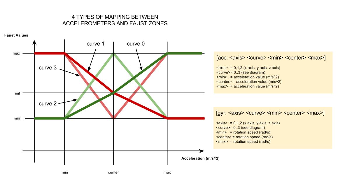
For example, controlling the gain of a synthesizer using the X axis of the accelerometer can be easily done simply by writing something like:
g = nentry("gain[acc: 0 0 -10 0 10]",0.5,0,1,0.01);
With this configuration, g = 0 when the device is standing vertically on its right side, g = 0.5 when the device is standing horizontally with screen facing up, and g = 1 when the device is standing vertically on its left side. Here is a working example:

Finally, in this slightly more complex mapping, g = 0 when the device is tilted on its right side and the value of g increases towards 1 when the device is tilted on its left side:
g = nentry("gain[acc: 0 0 0 0 10]",0,0,1,0.01);
Complex nonlinear mappings can be implemented using this system.
Widget Modulation
Widget modulation acts on the widgets of an existing Faust expression, but without requiring any manual modifications of the expression's code. This operation is done directly by the compiler, according to a list of target widgets and associated modulators. Target widgets are specified by their label, as used in the graphical user interface. Modulators are Faust expressions that describe how to transform the signal produced by widgets. The syntax of a widget modulation is the following:
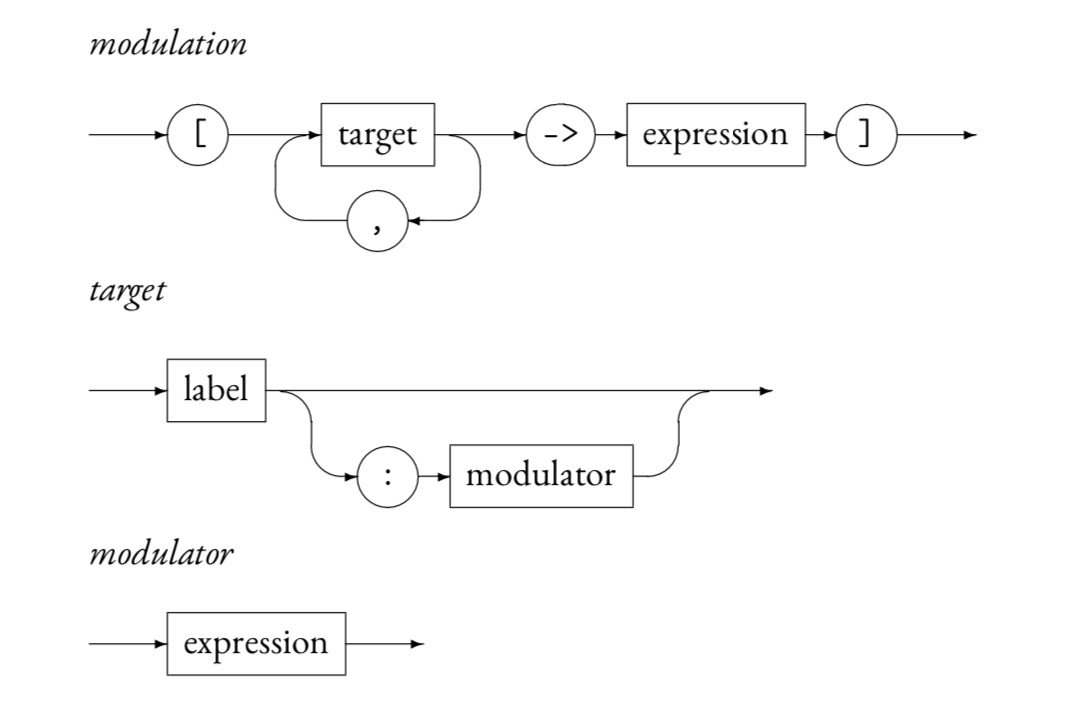
Here is a very simple example, assuming freeverb is a fully fonctional reverb with a "Wet" slider:
["Wet" -> freeverb]
The resulting circuit will have three inputs instead of two. The additional input is for the "Wet" widget. It acts on the values produced by the widget inside the freeverb expression. By default, the additional input signal, and the widget signal are multiplied together. In the following example, an external LFO is connected to this additional input:
lfo(10, 0.5), _, _ : ["Wet" -> freeverb]
Target Widgets
Target widgets are specified by their label. Of course, this presupposes knowing the names of the sliders. But as these names appear on the user interface, it's easy enough. If several widgets have the same name, adding the names of some (not necessarily all) of the surrounding groups, as in: "h:group/h:subgroup/label" can help distinguish them.
Multiple targets can be indicated in the same widget modulation expression as in:
["Wet", "Damp", "RoomSize" -> freeverb]
Modulators
Modulators are Faust expressions, with exactly one output and at most two inputs that describe how to transform the signals produced by widgets. By default, when nothing is specified, the modulator is a multiplication. This is why our previous example is equivalent to:
["Wet": * -> freeverb]
Please note that the ':' sign used here is just a visual separator, it is not the sequential composition operator.
To indicate that the modulation signal should be added, instead of multiplied, one could write:
["Wet": + -> freeverb]
Multiplications and addition are examples of 2->1 modulators, but two other types are allowed: 0->1 and 1->1.
Modulators with no inputs
Modulators with no inputs 0->1 completely replace the target widget (it won't appear anymore in the user interface). Let's say that we want to remove the "Damp" slider and replace it with the constant 0.5, we can write:
["Damp": 0.5 -> freeverb]
Modulators with one input
A 1->1 modulator transforms the signal produced by the widget without the help of an external input. Our previous example could be written as:
["Wet": *(lfo(10, 0.5)) -> freeverb]
If lfo had its user interface, it would be added to the freeverb interface, at the same level as the "Wet" slider.
Modulators with two inputs
Modulators with two inputs, like * or +, are used to combine the signal produced by the target widget with an external signal. The first input is connected to the widget, the second one is connected to the external signal. As we have already seen, our example could be written as:
lfo(10, 0.5), _, _ : ["Wet": * -> freeverb]
The main difference with the previous case is that if lfo had a user interface, it would be added outside of the freeverb interface. Please note that only 2->1 modulators result in additional inputs.
Here is a complete example:
